Machine Learning Algorithms
Key Takeaways
Machine learning algorithms are mathematical procedures that enable computers to learn patterns from data and make predictions, powering the vast majority of practical AI systems in 2026.
These algorithms are grouped into five main types: supervised learning, unsupervised learning, semi-supervised learning, self-supervised learning, and reinforcement learning, each suited to different data scenarios.
Classic algorithms like linear regression, decision trees, random forests, gradient boosting, and neural networks remain core tools in production systems from 2015 through 2026.
Newer paradigms such as self-supervised learning and large foundation models (including GPT-4-class systems) are trained with specialized algorithms built on these fundamentals.
Choosing the right algorithm depends on data labeling availability, problem type, and constraints like interpretability versus accuracy-and teams who follow focused information sources like KeepSanity AI can track real algorithmic breakthroughs without drowning in daily noise.
Introduction
Whether you're a data scientist, ML engineer, or student, understanding machine learning algorithms is essential for building effective AI systems and making informed technology choices. Machine learning algorithms are at the heart of artificial intelligence, enabling computers to learn from data, identify patterns, and make predictions without being explicitly programmed. This guide covers the main types of machine learning algorithms, how they work, and how to choose the right one for your project. By mastering these concepts, you'll be better equipped to select, implement, and evaluate the best solutions for real-world problems.
What Is a Machine Learning Algorithm?
Machine learning algorithms are sets of rules that allow computers to learn from data, identify patterns and make predictions without being explicitly programmed.
A machine learning algorithm is a mathematical procedure that transforms input data into a predictive or decision-making model. Unlike traditional software where programmers manually encode every rule, machine learning systems discover patterns directly from examples. You provide the data, the algorithm figures out the logic.
Most practical machine learning algorithms were introduced between the 1950s and 2010s, and they remain heavily used today. The perceptron emerged in 1958 as an early neural network for binary classification. Backpropagation, popularized in the 1980s by Rumelhart, Hinton, and Williams, enabled efficient training of multi-layer networks. Leo Breiman formalized random forests in 2001, and XGBoost appeared around 2014, quickly becoming a staple in production systems. These aren’t museum pieces-they power real applications in 2026.
The core workflow looks like this: training data goes in, the learning algorithm processes it to produce a trained machine learning model, and that model generates predictions on new data. For example, in credit scoring workflows using 2020–2025 banking datasets, an algorithm like logistic regression ingests features such as payment history, debt-to-income ratios, and account age. The training process finds optimal weights that map these input variables to default probabilities. The resulting model then scores new applicants in real time.
It’s worth clarifying the distinction between “algorithm” and “model.” The algorithm is the learning procedure-like gradient descent minimizing a loss function. The model is the learned parameters-the actual weights stored after training a 2024 fraud detection system. The algorithm tells you how to learn; the model is what you learned.
This article focuses on the main families of machine learning methods used in real systems: supervised learning algorithms, unsupervised learning algorithms, semi-supervised learning, self-supervised learning, reinforcement learning algorithms, and ensemble methods that improve base learners.
Types of Machine Learning Algorithms
Before diving into specific algorithms, it helps to understand the major categories. Each type addresses different data scenarios and problem structures.
Supervised learning: Learns from labeled training data (input-output pairs) to predict outcomes for new examples. Used for classification tasks and regression tasks.
Unsupervised learning: Finds structure in unlabeled data without predefined outputs. Used to identify patterns, group similar items, and reduce complexity.
Semi-supervised learning: Combines a small amount of labeled data with a large amount of unlabeled data to improve learning efficiency.
Self-supervised learning: Generates its own labels from the data itself (e.g., predicting masked words), enabling training on massive unlabeled datasets.
Reinforcement learning: Learns to make sequential decisions by interacting with an environment and receiving rewards.
In modern AI stacks-especially 2023–2026 large language models-these types are often combined. A system might use self-supervised pretraining on massive text corpora, supervised fine-tuning on task-specific labeled data, and reinforcement learning from human feedback (RLHF) for alignment.
The following sections dive into concrete algorithms in each category, mirroring how a data scientist actually chooses tools for projects.
Supervised Learning Algorithms
Supervised learning is the workhorse of applied machine learning. According to industry benchmarks through 2026, supervised methods account for over 70% of production ML deployments in business contexts. The core idea is simple: you have labeled examples showing the correct output for each input, and the algorithm learns to replicate that mapping.
Typical tasks include fraud detection in transaction logs, medical diagnosis on 2015–2024 hospital data, customer churn prediction, and demand forecasting. Supervised learning algorithms are usually split into classification algorithms for discrete labels (fraud vs. non-fraud) and regression algorithms for continuous values (predicted revenue, temperature forecasts).
Evaluation uses metrics appropriate to the task: accuracy for balanced classification, F1-score for imbalanced classes, root mean squared error (RMSE) for regression, and AUC-ROC for probabilistic classifiers.
The key supervised algorithms covered below include linear regression, logistic regression, decision trees, k-nearest neighbors, Naive Bayes, support vector machines, random forest, gradient boosting, and feed-forward neural networks.
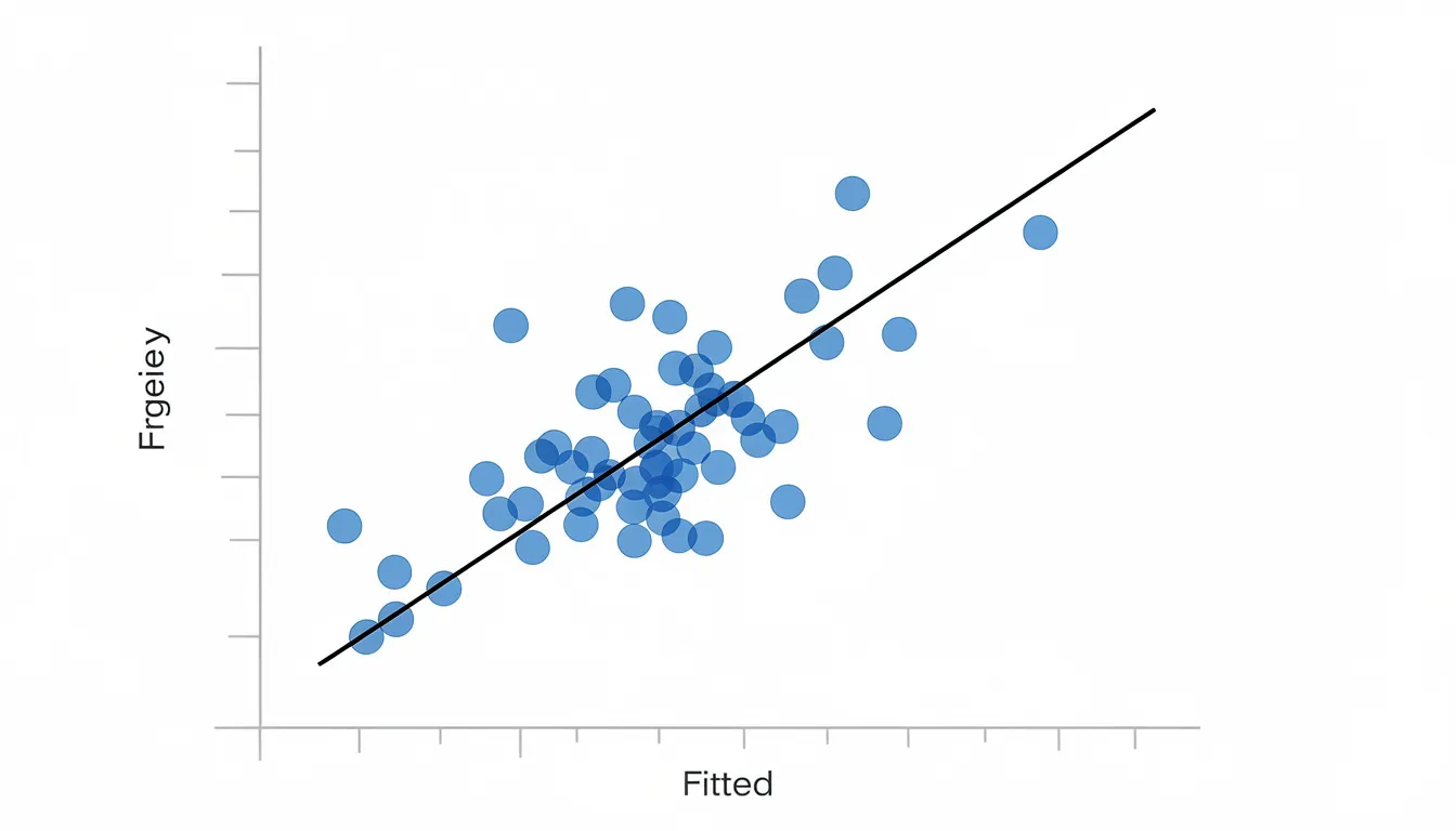
Linear Regression
Linear regression is one of the oldest and most widely used algorithms for predicting continuous values. The core idea dates back to early 1900s statistical work, with modern machine learning formalization developing through the 20th century.
The algorithm fits a straight line (or hyperplane in higher dimensions) through your data points, minimizing the squared error between predictions and actual values. If you’re forecasting monthly sales for a 2022–2026 e-commerce site based on advertising spend and seasonality, linear regression finds the relationship between those input variables and revenue.
Several variants address different challenges:
Multiple linear regression: Handles multiple independent variables simultaneously
LASSO (L1 regularization): Popularized in the 1990s by Tibshirani, induces sparsity for feature selection
Ridge regression (L2): Formalized in the 1970s by Hoerl and Kennard, addresses multicollinearity
Linear regression trains in milliseconds even on millions of rows, making it ideal for rapid iteration. The coefficients are directly interpretable-you can explain exactly how each feature affects the dependent variable.
Linear regression remains a strong baseline for tabular datasets in business and economics. Start here before reaching for complex models.
Logistic Regression
Despite its name, logistic regression is a classification algorithm, not a regression one. Developed in the 1950s–1960s for bioassay analysis, it maps inputs to probabilities between 0 and 1 using a sigmoid curve.
For binary classification tasks like “churn / no churn” or “fraud / not fraud,” logistic regression outputs the probability that an example belongs to the positive class. A threshold (commonly 0.5) converts these probabilities to class labels.
Extensions include:
Multinomial logistic regression: Handles multi-class problems via softmax
Regularized logistic regression: Uses L1/L2 penalties for high-dimensional features like text bag-of-words representations
Logistic regression is particularly popular in regulated domains. In finance (2010s–2020s) and healthcare studies through 2026, auditors and clinicians need to understand exactly how the model makes decisions. The coefficients directly show each feature’s impact-a positive coefficient on high debt indicates increased default risk.
A concrete example: predicting loan default risks from 2018–2023 credit histories, where the model outputs a probability and the bank sets a threshold based on their risk tolerance.
Decision Trees
Decision trees are tree-structured models that recursively split data based on feature values. Early algorithms like ID3 (1986), C4.5 (1993), and CART (1984) established the foundation.
Each internal node represents a question about a feature (e.g., “income > $60,000?”). Branches represent the possible answers, and leaf nodes contain the final prediction. The tree learns which questions to ask by optimizing impurity measures like Gini or entropy.
Decision trees handle:
Both classification tasks and regression tasks
Mixed data types (numerical and categorical)
Missing values via surrogate splits
The main advantage is interpretability. Non-technical stakeholders can follow the logic from root to leaf. A 2021 retail company might use a decision tree to classify customers into risk tiers based on spending behavior-and explain exactly why each customer landed in their tier.
The downside: single trees can overfit without proper pruning or minimum leaf size constraints. This limitation led to ensemble methods like random forests.
k-Nearest Neighbors (k-NN)
k-NN is an instance-based method from the 1960s that makes predictions based on similarity. For a new data point, it finds the k closest training examples and predicts based on their majority class (classification) or average value (regression).
“Closeness” is measured using distance metrics like Euclidean distance:
d(x,y) = √Σ(xi - yi)²
k-NN is simple and often serves as a baseline for recommendation-style tasks. For example, recommending similar products based on a user’s browsing history on a 2024 e-commerce platform.
Key characteristics:
Training: Nearly instantaneous (just stores the data set)
Prediction: Can be slow (must search across all stored examples)
Scaling: Struggles with high dimensional data beyond 10-20 features (curse of dimensionality)
Preprocessing: Requires normalized feature scales
Naive Bayes
Naive Bayes is a family of probabilistic classifiers based on Bayes’ Theorem, with the “naive” assumption that features are conditionally independent given the class.
The variants address different data types:
Variant | Data Type | Typical Use |
|---|---|---|
Gaussian | Continuous | General classification |
Multinomial | Counts (TF-IDF) | Text classification |
Bernoulli | Binary | Document presence/absence |
Despite the naive independence assumption, these classifiers perform surprisingly well for spam detection, sentiment analysis on 2015–2024 social media data, and document tagging. Training completes in milliseconds even on large vocabularies.
Compared to transformers, Naive Bayes won’t match state-of-the-art accuracy on complex NLP tasks. But for speed and simplicity-especially when you need calibrated probability estimates quickly-it remains a practical choice in many machine learning systems.
Support Vector Machines (SVM)
Support vector machines are margin-based classifiers developed in the 1990s by Vapnik and colleagues. The core idea: find the hyperplane that separates classes with the maximum margin.
The “support vectors” are the critical data points closest to the decision boundary. These points alone determine the optimal hyperplane-you could remove all other training examples and get the same result.
Kernel functions extend SVMs to handle non-linear separation:
Linear kernel: For linearly separable data
Polynomial kernel: For polynomial decision boundaries
RBF (Radial Basis Function): For complex, non-linear patterns
SVMs were state of the art for many text and image classification tasks in the 2000s. They remain competitive on small to medium-sized datasets in 2026, with strong theoretical guarantees from PAC-learnability theory.
A practical example: classifying malware vs. benign software using a 2019–2024 cybersecurity data set, where SVMs can achieve high precision on extracted features.
The trade-offs: SVMs scale poorly on very large datasets (O(n²–n³) training time) and are less interpretable than trees or linear models.
Random Forest
Random forest is an ensemble of decision trees introduced in 2001 by Leo Breiman. It combines bagging (bootstrap aggregation) with random feature selection to create diverse, uncorrelated trees.
The process:
Create multiple bootstrap samples from training data (~63% unique rows per tree)
Train a decision tree on each sample, considering only a random subset of features at each split
Combine predictions via majority vote (classification) or averaging (regression)
Random forests reduce overfitting compared to single trees and have been a go-to baseline on tabular data in Kaggle competitions from 2012–2024. Use cases include credit scoring, churn prediction, and medical risk models.
Practical considerations:
Decent performance out of the box with minimal tuning
Moderate training time, parallelizable across trees
Good handling of non-linearities and feature interactions
Feature importance metrics available for interpretability
The random forest algorithm excels when you need a robust, reliable model without extensive hyperparameter optimization.
Gradient Boosting and Boosted Trees
Gradient boosting is a sequential ensemble method that adds models one by one, each correcting the residual errors of the previous ensemble. The technique was popularized in the late 1990s and early 2000s, with modern libraries making it accessible to practitioners.
Library | Released | Key Innovation |
|---|---|---|
XGBoost | 2014 | Regularized objectives, second-order approximations |
LightGBM | 2017 | Histogram binning, leaf-wise growth |
CatBoost | 2017 | Ordered boosting, native categorical handling |
These libraries dominate structured-data competitions and real-world systems. In 2017–2023 click-through rate prediction at major tech companies, gradient boosting consistently achieved AUCs of 0.85+ compared to 0.78 for single models.
Trade-offs:
Accuracy: Among the highest for tabular data
Flexibility: Handles various loss functions
Sensitivity: Requires careful hyperparameter tuning (learning rate 0.01–0.3, depth 3–10, n_estimators 100–10,000)
Overfitting risk: Higher than random forests without proper regularization
Example: an online marketplace in 2025 uses XGBoost to rank search results by relevance and conversion probability, blending user behavior signals with product attributes.
Neural Networks (Multilayer Perceptron)
Feed-forward neural networks, or multilayer perceptrons (MLPs), learn complex non-linear mappings through layers of neurons and activation functions. Formalized with backpropagation in the 1980s, they became the foundation for modern deep learning.
Basic structure:
Input layer: Receives feature values
Hidden layers: One or more layers of neurons with activation functions (ReLU since ~2010, where f(x) = max(0, x))
Output layer: Produces predictions
Weights are learned through gradient descent variants. Adam (introduced in 2014 by Kingma and Ba) with adaptive moment estimation became a default optimizer for many tasks.
While deep neural networks drive state-of-the-art results in computer vision and natural language processing, simpler MLPs are used for:
Credit scoring and fraud detection
Recommendation systems
Sensor data modeling
Tabular prediction when trees plateau
Example: predicting default probability using a two-hidden-layer MLP (512 → 128 neurons) trained on bank transactions from 2019–2024.
The artificial neural network architecture is also the building block for more advanced structures like CNNs, RNNs, and transformers that power 2018–2026 deep learning systems.

Unsupervised Learning Algorithms
Unsupervised learning works on unlabeled data to discover structure, groupings, or low-dimensional representations. This is crucial in domains where labels are scarce or expensive-think 2020–2026 cybersecurity logs, IoT sensor streams, or massive customer event datasets.
Key categories:
Clustering algorithms: Group similar data points together
Dimensionality reduction algorithms: Compress data into fewer features
Association rule learning: Discover co-occurrence patterns
Typical applications include market segmentation, anomaly detection, visualization of high dimensional data, and pattern discovery in transaction logs.
When do practitioners reach for unsupervised methods? Generally when:
Labels don’t exist or would cost thousands per expert annotation
You need to explore data structure before building supervised models
Visualization is the primary goal
You’re looking for unusual patterns (fraud, intrusion, equipment failure)
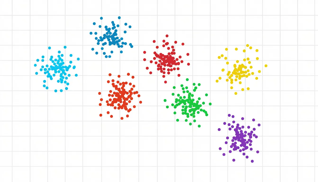
Clustering Algorithms
Clustering groups data points so that items in the same cluster are more similar to each other than to those in other clusters. It answers the question: “What natural groupings exist in my data?”
K-means (Lloyd’s algorithm, 1950s–1960s) is the most widely used centroid-based approach:
Initialize k centroids randomly
Assign each data point to the nearest centroid
Update centroids as the mean of assigned points
Repeat until convergence (typically 10–50 iterations)
Choosing k often uses the elbow method (plotting within-cluster sum-of-squares) or silhouette analysis.
Other clustering families:
DBSCAN (1996): Density-based, handles arbitrary cluster shapes and noise. Each data point belongs to a cluster based on neighborhood density, not distance to centroids.
Hierarchical clustering: Builds dendrograms for flexible cluster counts without predefining k
Concrete use cases:
Customer segmentation for a 2023 subscription app (identifying behavior-based tiers)
Network intrusion pattern discovery in 2020–2025 security logs
Grouping news articles by topic
Dimensionality Reduction Algorithms
Dimensionality reduction simplifies high dimensional data into fewer features, making models faster, less prone to overfitting, and easier to visualize.
Principal Component Analysis (PCA), dating to the early 20th century, is the core linear technique:
Finds directions (principal components) of maximum variance
Projects data onto these orthogonal components
Typically retains 95% of variance in 10–50 dimensions from 1000+ original features
Modern non-linear methods for visualization:
Method | Year | Approach |
|---|---|---|
t-SNE | 2008 | Minimizes KL-divergence on pairwise similarities |
UMAP | 2018 | Manifold approximation preserving topology |
These are widely used between 2015–2026 to visualize embeddings from deep models in 2D or 3D. When you see those beautiful cluster plots of language model embeddings, you’re usually looking at t-SNE or UMAP projections.
Use cases:
Reducing thousands of image pixels to tens of components
Visualizing 2023–2026 language model embeddings
Speeding up downstream supervised models
Exploratory data analysis before modeling
Association Rule Learning
Association rule learning discovers “if A then B” relationships in large transactional datasets. The classic example: market basket analysis revealing that customers who buy milk and bread often buy eggs.
Key metrics:
Support: What fraction of transactions contain the itemset?
Confidence: Given A, how often does B occur?
Lift: How much more likely is B given A, compared to B alone?
Canonical algorithms:
Apriori (1994): Generates candidate itemsets, prunes by support
FP-Growth (2000): Uses prefix trees for efficient mining without candidate generation
ECLAT (1997): Vertical data format for intersection-based counting
Practical applications in 2018–2024:
Supermarket basket analysis for cross-selling strategies
Clickstream navigation patterns on e-commerce sites
IoT event co-occurrence in smart home systems
Association rules translate directly to business actions. If {diapers} → {beer} has high lift, place them near each other. If certain page sequences lead to conversion, optimize that flow.
Semi-Supervised and Self-Supervised Learning
Real-world datasets in 2026 typically contain a small labeled subset and a massive unlabeled portion. Labeling is expensive-especially when it requires domain experts. This reality drives hybrid approaches that leverage both labeled and unlabeled data.
Semi-supervised learning algorithms combine the two: use limited labeled data to guide learning while letting unlabeled examples refine the decision boundary. Techniques like label propagation and consistency regularization can boost accuracy 5–20% compared to using labeled data alone.
Self-supervised learning takes a different approach: generate labels automatically from the data itself. Mask a word and predict it. Remove a patch from an image and reconstruct it. These pretext tasks create massive training signals without human annotation.
Self-supervised pretraining underpins modern foundation models deployed by 2026. When you use a large language model or a pretrained vision encoder, you’re benefiting from self-supervised algorithms.
Semi-Supervised Learning Algorithms
Semi-supervised learning precisely addresses scenarios like: you have 10,000 labeled medical images but 1 million unlabeled ones from the same distribution. How do you use all the data?
Classic methods:
Self-training: Train on labeled data, use confident predictions as pseudo-labels for unlabeled examples, retrain
Label propagation (Zhu, 2003): Build a similarity graph, propagate labels through connected nodes
Co-training (Blum/Mitchell, 1998): Train on different views of the data, let each model label examples for the other
Modern deep semi-supervised techniques:
Consistency regularization: Augmented versions of the same input should produce similar predictions
MixMatch (2019): Combines consistency regularization, entropy minimization, and MixUp augmentation
These appeared in 2020–2025 benchmarks for image classification, often matching fully-supervised performance with 10x fewer labels.
Applications where labeling is expensive:
Radiology scans requiring radiologist review
Legal document classification needing lawyer expertise
Niche industrial sensor data with rare failure modes
The intuition: unlabeled data reveals the structure of the input space. The decision boundary should pass through low-density regions, not through clusters of similar examples.
Self-Supervised Learning Algorithms
Self-supervised learning constructs surrogate tasks from unlabeled data. The model learns useful representations while solving these pretext tasks-then transfers to downstream applications.
Text examples:
Next-token prediction: GPT-style models (GPT-2 in 2019, GPT-3 in 2020, GPT-4-class systems by 2023) predict the next word given context
Masked language modeling: BERT (2018) predicts 15% of masked tokens in a sentence
Vision examples:
Contrastive learning: SimCLR (2020), MoCo (2019) maximize agreement between augmented views of the same image
BYOL (2020): Bootstrap representations without negative samples
Masked autoencoders (2021): Reconstruct masked image patches
The impact is dramatic. Self-supervised pretraining on massive unlabeled corpora (2010–2024 web text, photo collections) creates representations that transfer to downstream tasks with minimal labeled data. Fine-tuning a pretrained model on 1,000 labeled examples often beats training from scratch on 100,000.
Understanding these algorithms is key to grasping how modern AI assistants and multimodal models reached their 2023–2026 performance levels.
Reinforcement Learning Algorithms
Reinforcement learning addresses sequential decision-making: an agent interacts with an environment, receives rewards, and learns a policy that maximizes long-term returns. Unlike supervised learning with static labeled examples, RL learns from trial and error.
Iconic milestones:
TD-Gammon (1990s): Tesauro’s backgammon program
DQN (2013–2015): DeepMind beating Atari games at human level
AlphaGo (2016): Defeating world champion Lee Sedol
RLHF (2022–2024): Aligning language models via human preference feedback
The core elements:
Agent: The learner/decision-maker
Environment: What the agent interacts with
State: Current situation
Action: What the agent can do
Reward: Feedback signal
Policy: Strategy mapping states to actions
RL is powerful but data-hungry and complex to deploy. It tends to be used in high-value domains (ad bidding, robotics) or where simulation is cheap (games, recommendation loops).
Model-Free Reinforcement Learning Methods
Model-free RL learns directly from experience without modeling environment dynamics. You don’t need to know how the world works-just what happens when you take actions.
Value-based methods estimate expected returns:
Q-learning (1989): Tabular method learning Q(state, action) values
Deep Q-Networks (DQN, 2013–2015): Neural network for high-dimensional states, with experience replay and target networks for stability
Policy-based and actor-critic methods directly optimize the policy:
REINFORCE (1992): Policy gradient method using Monte Carlo returns
Proximal Policy Optimization (PPO) (2017): Clipped objective for stable updates, widely used in 2018–2025 robotics and game AI
Real-world use cases:
Optimizing ad bidding policies (10–30% ROI improvements)
Controlling robots in warehouse automation
Refining conversational models via RLHF
Game AI and autonomous systems
Practical challenges remain significant: exploration vs. exploitation, sample efficiency (often needing millions of timesteps), safety constraints, and the need for realistic simulators when live experimentation is risky.
Ensemble Learning: Bagging, Boosting, and Stacking
Ensemble learning combines multiple base models to achieve better performance and robustness than any single model. The principle: diverse weak learners, properly aggregated, can form strong learners.
Ensemble methods became standard toolbox techniques during 2000–2020 and remain core in enterprise ML platforms in 2026. They’re especially useful on noisy tabular data and in high-stakes prediction tasks where incremental accuracy gains matter.
The three main paradigms:
Bagging: Train models in parallel on different data samples
Boosting: Train models sequentially, each focusing on previous errors
Stacking: Train a meta-model on base model predictions
Ensembles often win ML competitions but can be harder to interpret, pushing teams to use model explainability tools like SHAP or LIME alongside them.
Bagging (Bootstrap Aggregation)
Bagging trains many models in parallel on different bootstrap samples (random samples with replacement) of the training data. Predictions are aggregated via voting (classification) or averaging (regression).
The classic ensemble learning algorithm using bagging is random forest:
Each tree sees ~63% unique training examples
Each split considers a random subset of features (√p for classification)
Hundreds of trees vote on the final prediction
Bagging reduces variance-the instability that causes decision trees to overfit. A single tree might memorize noise; an average of 500 trees smooths that out.
Example: bagged decision trees stabilizing churn prediction models for a telecom operator between 2017–2023, reducing false positive rates.
Pros and Cons of Bagging:
Pros | Cons |
|---|---|
Robust to overfitting | Larger model size |
Easy to parallelize | Less interpretable than single tree |
Handles noisy data well | Memory-intensive for many trees |
Boosting
Boosting trains weak learners sequentially, with each new model focusing on the mistakes of previous ones. The ensemble improves iteratively.
Key algorithms:
AdaBoost (1995): Reweights misclassified examples exponentially
Gradient Boosting (Friedman, 1999–2001): Fits new models to pseudo-residuals
XGBoost, LightGBM, CatBoost: Modern implementations with regularization and efficiency optimizations
Each new tree in gradient boosting is fit to the residual errors-the gap between current predictions and true values. With a small learning rate (0.01–0.1) and many iterations, the ensemble gradually converges to accurate predictions.
Adoption examples:
Ranking search results at major tech firms in the 2010s
Risk scoring in fintech start-ups from 2018–2025
Over 95% of tabular Kaggle competition winners use boosting
The ensemble learning method is powerful but demands careful tuning. Without proper regularization, boosting can overfit-especially with too many trees or too high a learning rate.
Stacking
Stacking (stacked generalization) trains diverse base models and then trains a meta-model on their predictions. The meta-learner learns how to weight or combine base learners to correct their biases.
Typical workflow:
Train logistic regression, random forest, gradient boosting, and neural network on training data
Generate predictions (or probabilities) from each base model
Train a simple meta-model (often logistic regression or linear regression) on these predictions as features
Use the stacked ensemble for final predictions
Stacking is common in competitions and some production recommendation systems. The gains are typically small (2–4 percentage points) but meaningful in high-stakes applications.
Related concept: knowledge distillation (Hinton, 2015), where a large ensemble “teacher” guides a smaller, faster “student” model-enabling deployment of ensemble-quality predictions at single-model latency.
Example: a 2024 fraud detection system stacks XGBoost, random forest, and MLP base models, using logistic regression as the meta-learner to optimize the precision-recall trade-off.
Architectures vs. Algorithms
It’s easy to conflate model architecture with training algorithm, but they’re distinct concepts:
Architecture: The structure of the model-layers, connections, attention mechanisms. Determines what the model can express.
Algorithm: The training procedure-loss function, optimizer, learning rule. Determines how parameters are discovered from data.
The same transformer architecture (introduced by “Attention Is All You Need” in 2017) can be trained with different algorithms for different purposes:
Training Approach | Task | Example |
|---|---|---|
Cross-entropy + teacher forcing | Translation | Machine translation models |
Next-token prediction | Text generation | GPT-series models |
Masked language modeling | Representation learning | BERT |
Contrastive + captioning | Multimodal | CLIP |
RLHF | Alignment | ChatGPT, Claude |
Changes in training objectives can radically change model behavior even when architecture is fixed. An autoencoder trained to minimize reconstruction loss learns compressed representations. Take the same encoder, add a classification head, fine-tune with cross-entropy-now it’s a classifier.
In 2023–2026 AI systems, this distinction matters. When someone says a model was “aligned using RLHF,” they’re describing the training algorithm, not the architecture. The transformer stayed the same; the learning procedure changed.
How to Choose a Machine Learning Algorithm
There is no universally best algorithm. The “no free lunch” theorem (Wolpert, 1997) formalizes this: any algorithm that performs well on one class of problems must perform worse on another. Practitioners choose based on data, problem type, resources, and constraints.
Key Selection Factors
Key selection factors include:
Type of data: Tabular (trees/boosting excel), images (CNNs/transformers), text (transformers, NB for simple tasks), time series (RNNs, gradient boosting)
Size of data set: Small datasets favor simple models; millions of rows enable complex methods
Label availability: Labeled data → supervised; unlabeled → unsupervised or self-supervised; mixed → semi-supervised
Interpretability requirements: Regulated domains may require trees or linear models
Latency and compute budget: Real-time serving may preclude large ensembles
Organizational expertise: What can your team actually deploy and maintain?
Concrete Guidance Patterns
Concrete guidance patterns for algorithm selection:
Scenario | Starting Algorithm |
|---|---|
Millions of tabular rows (2026) | LightGBM or XGBoost |
Small tabular dataset | Linear/logistic regression, decision trees |
High-dimensional images | Pretrained CNN or vision transformer |
Large text corpus | Pretrained transformer, fine-tuned |
Limited labels + lots of unlabeled data | Semi-supervised or transfer learning |
Sequential decisions | Reinforcement learning (if simulation available) |
Real-world example: selecting algorithms for a hospital readmission model might favor gradient boosting with SHAP explanations (clinicians need interpretability), while a recommendation widget tolerates neural network embeddings (users don’t need explanations).
Model evaluation via cross-validation and a held-out test set from recent data (2022–2024) is more reliable than theoretical expectations. Run experiments, not debates.
Applications of Machine Learning Algorithms in 2026
Machine learning algorithms underpin AI systems across every major sector. The market that was $91B is projected to reach $1.88T by 2035 (Itransition), driven by applications that deliver measurable business value.
Concrete 2018–2026 examples:
Fraud detection: SVMs and random forests achieving 99% precision on payment transactions
Healthcare diagnostics: CNNs reducing diagnostic error rates 5–10% on medical imaging
Spam and phishing filters: Naive Bayes algorithm and ensemble methods protecting billions of inboxes
Dynamic pricing: Gradient boosting optimizing airline and hotel rates in real-time
Personalized content feeds: Neural networks powering recommendation at streaming platforms
Energy optimization: Regression models reducing consumption in smart buildings
Predictive analytics: Time series models forecasting demand, maintenance, and inventory
Large language models and multimodal models combine several algorithmic ideas: self-supervised pretraining, supervised fine-tuning, RL for alignment, and sometimes ensemble distillation. They’re not replacements for classic algorithms-they’re built on top of them.
Staying current on which algorithms are actually shipping in products vs. which are research hype requires careful news filtering. Not every arXiv paper becomes production software.
Staying Sane While Following ML Algorithm Advances
Between 2018 and 2026, the volume of ML papers and algorithmic tweaks has exploded. ArXiv sees over 10,000 ML papers per year. Every week brings claims of “breakthrough” performance. Following everything directly from arXiv and social media is impossible-and counterproductive.
The typical problems with daily AI newsletters:
Sponsor-driven filler to justify ad rates
Minor updates framed as breaking news
Constant FOMO for practitioners who just want the signal
KeepSanity AI was created specifically to solve this problem. Instead of daily emails padded with noise, you get one weekly email focused only on major, enduring developments in AI and machine learning algorithms.
Curation principles:
No ads: No sponsor pressure to inflate minor updates
Signal only: Significant model or algorithm releases (major 2024–2026 foundational model papers, key RL breakthroughs)
Smart links: Papers linked to alphaXiv for easy reading
Scannable categories: Models, tools, business impact, robotics, trending papers
Lower your shoulders. The noise is gone. Here is your signal.
If you work with or study machine learning algorithms, consider adopting a “low-noise” information diet. Spend time understanding a few important machine learning techniques well, rather than skim-reading every minor update.

FAQ
Which machine learning algorithm should I learn first in 2026?
Start with linear regression, logistic regression, and decision trees using a mainstream machine learning library like scikit-learn. These algorithms are foundational, interpretable, and still widely used in production. They’ll teach you core concepts: loss functions, overfitting, feature engineering, and evaluation metrics. After grasping these, move to random forest and gradient boosting (XGBoost or LightGBM) for tabular data, then basic neural networks. Focus on data preprocessing and avoiding overfitting before tackling deep learning architectures. Following a weekly, curated AI update rather than daily feeds helps prioritize which newer algorithms deserve your study time.
How do I know if my dataset is big enough for complex algorithms?
Linear and tree-based models can deliver accurate predictions even with a few thousand labeled training examples. Deep neural networks and large transformers typically need tens of thousands to millions of examples to outperform simpler alternatives. Start with simple algorithms and cross-validation-if they underfit and you have substantial high-quality data, try more complex models. For images, audio, and text, transfer learning from pre-trained 2018–2026 models can compensate for smaller labeled datasets. Monitor learning curves (performance vs. dataset size) to determine when collecting more data beats changing algorithms.
Are classic algorithms still relevant now that we have large language models?
Absolutely. Classic algorithms like logistic regression, random forests, and gradient boosting remain heavily used in 2026 for structured business data, tabular risk models, and real-time production systems. Large language models excel at unstructured data-text, images, multimodal tasks-but are rarely the most efficient choice for straightforward tabular prediction. Many organizations run hybrid systems: LLMs for document understanding and conversations, classic ML for scoring, ranking, and forecasting. Understanding fundamentals makes it easier to reason about and safely deploy newer models.
What tools and libraries should I use to implement these algorithms?
For most supervised and unsupervised algorithms (regression, trees, SVMs, clustering, PCA), start with Python and scikit-learn as of 2026. For high-performance gradient boosting on tabular data, use XGBoost, LightGBM, or CatBoost. PyTorch and TensorFlow/Keras handle neural networks, deep learning algorithms, and self-supervised learning. For reinforcement learning techniques, explore Stable-Baselines3 or RLlib. Rely on curated resources-weekly AI digests and official documentation-to keep tooling knowledge current without chasing every minor library release.
How do I stay updated on important new machine learning algorithms without burning out?
Limit real-time feeds. Follow 1–2 trusted, low-noise sources that summarize significant developments weekly, focusing on breakthroughs rather than incremental tweaks. Scan paper digests linking to accessible summaries (like alphaXiv) and bookmark only algorithms that seem both novel and practically relevant to current projects. Set aside a fixed weekly time block-30–60 minutes every Friday-for catching up, rather than reacting to every headline. This approach mirrors the philosophy behind KeepSanity AI: protect attention, reduce FOMO, and invest time in deeply understanding key ideas instead of skimming dozens of shallow updates.