Algorithms for AI
Introduction
Artificial intelligence (AI) algorithms are the engines that drive modern intelligent systems, from chatbots and recommendation engines to fraud detection and robotics. This article provides a comprehensive overview of AI algorithms, their main types, and practical applications across industries. Whether you are a data scientist, engineer, or business leader, understanding the landscape of AI algorithms is essential for making informed decisions about technology adoption, model selection, and responsible deployment.
Scope:
We will cover the foundational concepts behind AI algorithms, explore the four major paradigms (supervised, unsupervised, semi/self-supervised, and reinforcement learning), and discuss how these algorithms are applied in real-world scenarios. The article also delves into key techniques such as optimization, dimensionality reduction, and ensemble methods, and addresses critical issues like bias, fairness, and responsible AI use.
Target Audience:
This guide is designed for data scientists seeking to deepen their technical knowledge, engineers building AI-powered systems, and business leaders who need to evaluate AI solutions or oversee AI-driven projects.
Why It Matters:
A clear understanding of AI algorithms empowers professionals to select the right tools for their needs, optimize performance, ensure compliance, and mitigate risks. As AI continues to transform industries, grasping the fundamentals of how these algorithms work is crucial for leveraging their full potential and ensuring ethical, effective deployment.
Key Takeaways
AI algorithms are concrete computational recipes-gradient descent, k-means, Q-learning-that power systems like GPT-4, Netflix recommendations, and fraud detection, fundamentally differing from traditional programming by learning patterns from data.
Most practical artificial intelligence today relies on four major paradigms: supervised learning algorithms (labeled data), unsupervised learning algorithms (pattern discovery), self-/semi-supervised learning (leveraging unlabeled data at scale), and reinforcement learning algorithms (trial and error with rewards).
Modern breakthroughs like transformers, large language models, and diffusion models share a few core algorithmic ideas: optimization through gradient descent, pattern recognition across massive datasets, and clever training setups that extract value from internet-scale unlabeled data.
Algorithm choice directly impacts cost, accuracy, and explainability-gradient-boosted trees still dominate tabular business data, while transformers handle unstructured text and images.
Staying informed matters: with new papers daily, curated low-noise sources like KeepSanity AI help teams track meaningful shifts without drowning in incremental tweaks.
What Is an AI Algorithm in Practice?
AI algorithms are mathematical instructions enabling computers to learn from data, classify information, and make predictions.
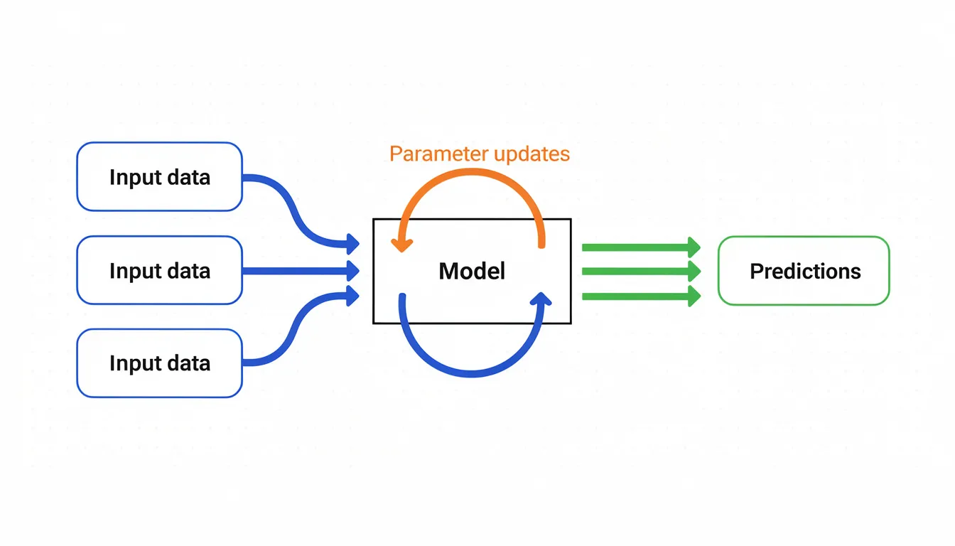
An AI algorithm is a step-by-step computational procedure that enables machines to learn patterns from data, make predictions, or optimize decisions. Unlike traditional fixed-rule programming where developers explicitly code every behavior, artificial intelligence algorithms iteratively adjust internal parameters based on feedback mechanisms like loss minimization or reward maximization.
Think of it this way: a classic algorithm might say “if transaction amount > $10,000, flag as suspicious.” An AI algorithm instead learns from thousands of transaction examples what combinations of features-amount, location, time, merchant type-actually predict fraud, discovering patterns no human programmer could specify in advance.
Concrete 2023-2025 Examples
In practice, here’s what ai algorithms work looks like across industries:
Gradient-boosted trees scoring credit risk: Banks use XGBoost and LightGBM to predict default probabilities, achieving AUC-ROC scores of 0.85-0.95 on datasets containing millions of loan applications. These machine learning models process input data like income, credit history, and employment status to generate accurate predictions.
Transformers powering GPT-4 and Gemini: These large language models use next-token prediction trained on trillions of tokens, with GPT-4 rumored to contain 1.76 trillion parameters. The learning process involves self-supervised pretraining followed by reinforcement learning from human feedback (RLHF).
Q-learning variants in robotics: OpenAI’s robotic systems and DeepMind’s game-playing agents use deep reinforcement learning to learn optimal actions through trial and error, updating value estimates via the Bellman equation.
What “Learning” Actually Means
When we say an algorithm “learns,” we mean it iteratively adjusts parameters to minimize a loss function (or maximize a reward). Here’s a concrete numeric example:
To fit a simple line y = mx + b to three data points-(1,2), (2,3), (3,5)-via gradient descent:
Start with m=0, b=0
Compute mean squared error (MSE) ≈ 2.67
Calculate gradients: ∂L/∂m ≈ 1.33, ∂L/∂b ≈ 0.67
Update with learning rate 0.1: m becomes -0.133, b becomes -0.067
Repeat until MSE drops below 0.01-typically under 100 iterations
This same principle-forward pass, loss evaluation, backward propagation of gradients, parameter update-scales from fitting a line to training models with billions of parameters.
Clarifying Terminology
These terms often get confused, but they mean different things:
Term | Definition | Example |
|---|---|---|
Algorithm | The training procedure or learning recipe | Adam optimizer, gradient descent, Q-learning |
Model | The instantiated function with learned parameters | A specific GPT-4 checkpoint with 1.76T parameters |
Architecture | The structural blueprint defining computation flow | Transformer’s multi-head attention layers |
Combined: transformer architecture + next-token-prediction objective + Adam optimizer = GPT-style LLM.
Core Families of AI Algorithms
Most AI systems in 2024 still fall into four major training paradigms: supervised learning, unsupervised learning, self-/semi-supervised learning, and reinforcement learning. Each uses training data and feedback differently, and understanding these distinctions helps you pick the right approach for your problem.
Here’s the key insight: many real-world systems combine several paradigms. ChatGPT, Claude, and Gemini all use self-supervised pretraining on massive text corpora, supervised fine-tuning on curated prompt-response pairs, and reinforcement learning from human feedback to align outputs with user expectations. OpenAI’s InstructGPT paper showed this hybrid approach boosted human preference rates from 70% to over 90%.
Supervised Learning Algorithms
Supervised learning algorithms require labeled datasets to train models by associating inputs with corresponding outputs.
Supervised learning trains on labeled data-input-output pairs where you already know the correct answer. The algorithm learns to map inputs to outputs, enabling classification (categorical outcomes) and regression (continuous values) on new data.
Practical business examples:
Email spam filters: Logistic regression on email metadata achieves 99% accuracy by learning which features (sender, keywords, links) predict spam
Credit scoring models: XGBoost predicting default probabilities with AUC-ROC of 0.85-0.95 on lending datasets
Click-through rate prediction: Advertising platforms use gradient-boosted trees to predict which ads users will click
Medical image diagnostics: Convolutional neural networks detecting early-stage cancer from radiology scans
Representative supervised learning algorithms:
Algorithm | Strengths | Best For |
|---|---|---|
Linear regression algorithm | Interpretable, fast | Baseline continuous prediction |
Logistic regression | Fast for millions of samples | Binary classification |
Decision trees | Intuitive splits | Explainable classification |
Random forest algorithm | Reduces variance, handles noise | General classification and regression problems |
XGBoost/LightGBM/CatBoost | Handles missing data, regularized | Tabular data competitions |
Feedforward neural networks | Scales to complex patterns | Large datasets with rich features |
The training loop works like this: a forward pass computes predictions, the loss function measures error (e.g., AUC for imbalanced classes, F1 for precision-recall tradeoffs in healthcare), backpropagation computes gradients via the chain rule, and optimizers update weights. This cycle repeats until the model’s predictions align with the labeled data.
For regulated domains like finance and healthcare, evaluation metrics matter enormously. Calibration curves verify that a model’s predicted probabilities match actual outcomes-critical when decisions affect human lives or financial stability.
Unsupervised Learning and Clustering Algorithms
Unsupervised learning algorithms analyze unlabeled data to identify patterns and correlations without predefined categories.
Unlike supervised learning, unsupervised learning algorithms discover structure in unlabeled data points without predefined categories. The algorithm identifies patterns humans might never think to specify.
Clustering algorithms are a subset of unsupervised learning that group data points based on similarity or proximity.
Clustering applications:
Customer segmentation: Marketing teams use k means clustering on RFM metrics (recency, frequency, monetary value) to group customers, often achieving 20-30% uplift in campaign ROI
Anomaly detection: DBSCAN detects intrusions in network traffic logs, spotting 95% of attacks without requiring labeled examples
Topic grouping: Hierarchical clustering organizes news archives by theme for exploratory data analysis
Key clustering algorithms:
Algorithm | How It Works | Best For |
|---|---|---|
K-means | Assigns data points to k centroids iteratively | Spherical clusters, fast processing |
DBSCAN | Density-based neighborhood detection | Arbitrary shapes, noise handling |
Hierarchical | Bottom-up agglomerative linkage | Dendrograms, topic grouping |
Gaussian Mixture Models | EM algorithm fitting probabilistic ellipsoids | Overlapping clusters |
Association rule mining extracts relationships from transactional data. The classic example: market-basket analysis revealing “customers who buy diapers often buy beer” with lift scores above 2, boosting cross-sales 15%. Algorithms like Apriori and FP-Growth make this computationally feasible on sparse transaction databases.
Clustering and association are often the first step in exploratory data analysis before deploying predictive models. Netflix, for example, clusters viewing histories before training supervised ranking models.
Self-Supervised and Semi-Supervised Learning Algorithms
Semi-supervised learning algorithms combine labeled and unlabeled data to improve model training efficiency and accuracy.
Self-supervised learning transforms unlabeled data into a supervised problem by creating pretext tasks-the algorithm predicts parts of the input from other parts, learning useful representations along the way.
Self-supervised approaches:
Masked language modeling (BERT): Predict 15% of masked tokens, yielding embeddings with 7-10% GLUE score improvements over unsupervised methods
Next-token prediction (GPT-3/4): Autoregressive language modeling at scale, enabling 175B+ parameter models with few-shot performance rivaling supervised approaches
Contrastive learning in vision (SimCLR, CLIP): Create augmented pairs of images, maximize agreement between representations-CLIP achieves 76% top-1 zero-shot accuracy across 26 datasets
Semi-supervised techniques combine a small labeled set with vast unlabeled data-practical when annotation is expensive, like medical imaging or legal document review.
Semi-supervised techniques:
Pseudo-labeling: Use model predictions above a confidence threshold as labels, iterate
Consistency regularization (MixMatch, FixMatch): Force predictions to stay consistent under augmentations, halving error on CIFAR-10 with just 250 labels
Graph propagation: Labels spread via personalized PageRank on similarity graphs
The impact is enormous: BERT’s pretraining on 3.3 billion words cut labeled data requirements 100x, powering an estimated 80% of production natural language processing systems by 2024 surveys.
Reinforcement Learning Algorithms
Reinforcement learning algorithms learn by interacting with an environment and receiving feedback in the form of rewards or penalties.
Reinforcement learning frames learning as trial and error with rewards. An agent interacts with an environment, takes actions, receives feedback, and learns policies that maximize cumulative reward over time.
Canonical algorithms:
Algorithm | Type | Notable Use |
|---|---|---|
Q-learning | Tabular, off-policy | Simple gridworld problems |
Deep Q-Networks (DQN) | Deep RL with CNNs | Atari games (from 10% to 100%+ human performance) |
Policy gradients (REINFORCE) | Samples trajectories | Continuous action spaces |
Actor-Critic (A2C, PPO) | Combines value and policy | RLHF in GPT-4, robotics |
Landmark achievements:
AlphaGo (2016) fused Monte Carlo Tree Search with deep value/policy networks, beating world champion Lee Sedol 4-1
AlphaZero self-played for just 4 hours to achieve superhuman performance in Go, Chess, and Shogi
GPT-4’s RLHF uses PPO to align a 1.5T+ parameter model on 50K+ human preference rankings
Practical 2020-2025 applications:
Dynamic pricing at Uber (RL bandits lifting revenue 5-10%)
Resource allocation in Amazon warehouses
Industrial control and robotics via sim-to-real transfer
Key challenges remain: sample inefficiency (often requiring 10^9 steps for proficiency), reward hacking, safety constraints, and bridging the gap between simulation and real world data.

Foundational Techniques Behind AI Algorithms
Beyond the four paradigms, several “building blocks” appear across nearly all machine learning algorithms: optimization, dimensionality reduction, and ensemble methods. Understanding these helps you see why certain approaches work and how practitioners tune them.
Optimization Algorithms
Gradient descent is the central algorithmic idea for training deep neural networks and many other models. The concept: iteratively adjust model parameters in the direction that reduces error, like walking downhill on a landscape where elevation represents loss.
Variants:
Batch GD: Full dataset per update (Stable but slow)
Stochastic GD: One sample per update (Noisy but fast)
Mini-batch GD: 32-512 samples per update (GPU sweet spot for deep learning)
Widely used optimizers:
SGD with momentum: Accelerates through plateaus
Adam: Adaptively scales learning rate per parameter via first/second moments (β1=0.9, β2=0.999)-enabled training ResNet-152 (2015) and transformers (2017+)
AdamW: Decouples weight decay, key for stable LLM training
RMSProp: Handles non-stationary objectives
Concrete example: Fitting a linear regression on a toy dataset [[1,2],[2,3],[3,5]] with learning rate 0.01, gradient descent converges MSE from 2.67 to 0.02 in roughly 500 steps. Modern systems add learning rate schedules (e.g., cosine annealing) and early stopping to prevent overfitting.
Dimensionality Reduction Algorithms
Dimensionality reduction maps high-dimensional data-like 768-dimensional text embeddings-into fewer dimensions while preserving meaningful structure. This speeds up training, enables visualization, and removes noise.
Key algorithms:
Algorithm | Approach | Best For |
|---|---|---|
Principal component analysis (PCA) | Orthogonal projection maximizing variance | Speed, production pipelines |
t-SNE | KL-divergence on pairwise similarities | Visualization (slow, O(n²)) |
UMAP | Topology-preserving fuzzy sets | Fast visualization, embeddings |
Autoencoders | Neural nets with bottleneck layers | Denoising, generative tasks |
Practical examples:
Visualizing customer segments in 2D scatter plots
Compressing embeddings for recommendation systems to reduce latency
Denoising sensor data in predictive maintenance (to predict equipment failures, data scientists often clean signals first)
While t-SNE and UMAP are often used only for exploratory plots, PCA and autoencoders can be part of production pipelines to accelerate inference.
Ensemble Algorithms
Ensemble learning combines multiple machine learning models to achieve better accuracy and robustness than any single model. The intuition: diverse models make different errors, and averaging them cancels mistakes out.
Bagging (Bootstrap Aggregating):
Random forest is the classic example. Train 100-500 decision trees on bootstrap samples of the data, then average predictions. This reduces variance and overfitting by a factor of √N, with out-of-bag error estimates for free.
Boosting:
Sequentially train models that focus on previous errors:
AdaBoost: Weights misclassified examples higher
Gradient Boosting: Fits new trees to residual errors
XGBoost: 108 binary classification wins on Kaggle benchmarks, with L1/L2 regularization and native missing data handling
LightGBM: 242 total wins, histogram-based for 10x speed on billion-row datasets
CatBoost: 243 wins, natively encodes categorical features without one-hot explosion
Stacking:
Train a meta-model on predictions from base learners. Combining XGBoost + neural net + logistic regression often yields 2-5% accuracy lift in competitions.
In 2024, ensembles still beat deep learning for credit scoring, churn prediction, and many tabular business analytics tasks where data is limited and interpretability matters.
Deep Learning Architectures vs. Algorithms
A common confusion: mixing up architectures (network structure) with algorithms (training procedures). The architecture defines how inputs flow through computations. The algorithm defines how parameters get updated.
Key deep learning families:
Architecture | Structure | Training Algorithm Examples |
|---|---|---|
CNNs | Convolutional filters + pooling | Supervised classification, contrastive learning |
RNNs/LSTMs | Gated recurrence for sequences | Next-step prediction, sequence labeling |
Transformers | Self-attention mechanisms | Next-token prediction, masked LM, RLHF |
Autoencoders/VAEs | Encoder-bottleneck-decoder | Reconstruction loss, KL divergence |
Diffusion models | Iterative denoising | DDPM noise prediction |
Identical architectures can perform different tasks depending on objectives. A transformer can be a language model (GPT), a classifier (fine-tuned BERT), or an encoder for retrieval systems (sentence transformers). The training algorithm-next-token prediction vs. contrastive learning vs. classification loss-defines the behavior.
Transformers and Large Language Models (LLMs)
The transformer architecture, introduced in Vaswani et al.’s 2017 “Attention is All You Need” paper, became the backbone of modern NLP and multimodal AI systems.
Core algorithmic ideas:
Self-attention: Dynamically weights the relevance of all input tokens to each other, enabling parallel processing of sequential data
Positional encoding: Sine/cosine functions inject sequence order information
Scaling laws: Loss decreases predictably with compute-Chinchilla (2022) showed loss ~ compute^{-0.095}
Self-attention allows transformers to process long-range dependencies, outperforming recurrent neural networks by factors of 10x in training speed on GPUs.
Next-token prediction is the central objective behind GPT-3 (2020), GPT-4 (2023/2024), Google Gemini (2023), and Meta’s Llama series (2023-2024). At 100B+ parameters, models show emergent capabilities like zero-shot reasoning that don’t appear in smaller versions.
The LLM training stack:
Pretraining: Self-supervised on trillions of web tokens
Instruction fine-tuning: Supervised on 10K+ curated prompt-response pairs
RLHF: Reward model trained on human rankings, PPO optimizes policy
Retrieval-augmented generation (RAG) combines LLMs with vector search. Instead of relying solely on parametric knowledge, the model retrieves relevant documents via FAISS or similar systems, stuffs them into context, and generates grounded responses-cutting hallucination rates 30-50%.
Other Modern Architectures: CNNs, Autoencoders, and Diffusion Models
Convolutional neural networks remain the default for image tasks in many production systems. Pre-vision-transformers, CNNs powered:
Early medical imaging AI (detecting diabetic retinopathy)
Object detection in self-driving cars (YOLO, Faster R-CNN)
Quality control in manufacturing (defect classification)
ResNet-50 achieved 1.2% ImageNet top-5 error in 2015, and these architectures still run in edge deployments where latency and cost matter.
Autoencoders and VAEs compress and reconstruct data through bottleneck layers. Uses include:
Denoising corrupted inputs (robust to 20% noise)
Dimensionality reduction for downstream tasks
Generative modeling via the VAE’s probabilistic latent space
Diffusion models (DDPMs) underpin Stable Diffusion (2022), Midjourney, and DALL·E series. The algorithmic idea: add Gaussian noise over T=1000 steps, then train a neural network to reverse the process. Stable Diffusion generates 512x512 images in roughly 50 denoising steps using classifier-free guidance.
Multimodal models now combine these architectures-transformers handling text, diffusion handling images, sometimes sharing representations across modalities.

How AI Algorithms Learn: Training Setups and Data Regimes
Beyond the algorithm itself, how you present data over time matters enormously for cost, responsiveness, and performance. The same gradient descent can be deployed in different regimes depending on your constraints.
Batch, Online, and Incremental Training
Batch training processes the full dataset (or large chunks) in epochs. This is dominant for deep learning-training GPT-4 on trillions of tokens or ResNet on ImageNet requires stable, repeatable passes through the data.
Online training updates the model with each new data point or tiny batch. Applications include:
Ad bidding systems adapting in milliseconds
Anomaly detection responding to new threat patterns
Recommendation systems tracking user behavior shifts
Incremental training falls between: periodic updates (nightly, weekly) using newly collected data. Email spam filters recalibrate on fresh examples; risk models update monthly with recent defaults.
Training Mode | Update Frequency | Example Use Case |
|---|---|---|
Batch | Full epochs | LLM pretraining, image classification |
Online | Per-sample or micro-batch | Real-time ad targeting |
Incremental | Scheduled (daily/weekly) | Spam filters, fraud models |
Trade-offs involve computational cost, responsiveness to drift, and deployment complexity. Teams often start with batch training and add incremental updates as scale grows.
Transfer Learning and Pretrained Models
Transfer learning reuses knowledge from models trained on massive, generic datasets-ImageNet for vision, Common Crawl for text-and fine-tunes them on smaller, task-specific data.
Examples:
Fine-tuning BERT for legal contract classification (95% accuracy vs. 80% training from scratch)
Adapting a pre-trained ResNet for manufacturing defect detection
Customizing Llama-2-70B for internal document Q&A, slashing costs 100x
The algorithmic steps:
Load pretrained weights
Freeze or partially freeze early layers
Attach a new output head for your task
Train for a few epochs on your labeled data
Benefits include reduced compute cost, better performance with limited labels, and faster experimentation-critical for smaller teams and startups.
The 2022-2025 boom in open-source models (Llama, Mistral, Stable Diffusion checkpoints) made transfer learning more accessible than ever. You no longer need Google-scale resources to build competitive AI systems.
Choosing and Applying Algorithms Without Losing Your Sanity
With hundreds of named artificial intelligence algorithms, how should a team in 2024-2026 decide what to actually use? The answer isn’t “try everything.” It’s starting from your constraints and working backward.
Rule-of-thumb guidance:
Data Type | Size | Recommendation |
|---|---|---|
Tabular | <100K rows | Gradient-boosted trees (XGBoost, CatBoost) |
Tabular | >1M rows | LightGBM or neural nets |
Text/Images | Any | Transformers with transfer learning |
High interpretability needed | Any | Logistic regression, decision trees |
Latency-critical | Any | Simpler models, distillation |
Non-technical constraints matter equally: GDPR requires explainability (pushing teams toward SHAP values), compute budgets limit deep learning experiments, and annotation costs make self-supervised approaches attractive.
Case Study: Churn Prediction
A mid-size SaaS company evaluated algorithms for customer churn:
Logistic regression baseline: AUC = 0.75, fully interpretable
XGBoost: AUC = 0.82, feature importance via SHAP
Neural network: AUC = 0.80, black-box
They chose XGBoost-slightly better accuracy than the neural net, plus regulatory-friendly explanations for customer communications. The marginal accuracy loss was worth the maintainability gain.
In a landscape where new ai algorithms learn variations appear in papers daily, curated sources matter. KeepSanity AI delivers one email per week with only major developments-no daily filler, no sponsored noise. When a breakthrough like AdamW2 halves training time, you’ll know. When minor tweaks don’t matter, you won’t waste time reading about them.
From Business Problem to Algorithm Shortlist
A concrete decision flow:
Define objective and constraints: Classification? Regression? Ranking? What latency is acceptable? What’s the explainability requirement?
Profile your data: How many rows? Labeled or unlabeled? Structured or unstructured? Time series or static?
Shortlist algorithm families:
Tabular classification with limited data → gradient-boosted trees
Large text corpus → transformer-based models (fine-tune BERT, Llama)
Sequential decision-making → RL or contextual bandits
Mostly unlabeled → self-supervised pretraining first
Benchmark baselines: Start with logistic regression, random forest, XGBoost before adopting complex architectures. Often the simple model wins.
Validate properly: Keep a holdout set, perform cross-validation, watch for data leakage (especially in time series where future information can leak into training).
Simplicity aids maintainability. A marginally weaker model that’s easier to monitor and debug is often the right production choice.
Monitoring, Drift, and Model Lifecycle
Models degrade. User behavior shifts after product launches. Economic conditions change credit risk profiles. Fraud patterns evolve.
Types of drift:
Concept drift: The relationship between inputs and outputs changes (COVID shifted credit risk by 20%)
Data drift: Input distributions shift (seasonal changes in e-commerce)
Basic monitoring metrics:
Prediction distributions over time
Calibration curves and error rates
Performance by subgroup (catching fairness issues)
Set up scheduled retraining-nightly for fast-moving domains, monthly for stable ones-with triggers based on KS-test distribution shifts exceeding 0.1 or performance thresholds breaching acceptable bounds.
Algorithm choice influences monitoring needs: RL systems require reward tracking; LLMs using RAG need retrieval quality checks alongside generation metrics.
As new techniques for drift detection, monitoring, and alignment emerge, practitioners benefit from curated updates rather than daily noise. That’s where a weekly digest like KeepSanity AI helps-you get the signal on what’s actually changed without losing your focus to minor incremental papers.

Risks, Bias, and Responsible Use of AI Algorithms
Algorithmic power without guardrails leads to bias, opacity, and misuse. The 2023-2025 period saw significant regulatory moves: the EU AI Act establishing risk tiers, US AI-related executive orders mandating safety testing, and growing stakeholder pressure for transparency.
Risk doesn’t come only from “bad data.” Even mathematically elegant algorithms can produce unfair outcomes or be exploited if context is ignored. Treat responsible AI considerations as core design constraints, not compliance afterthoughts.
Bias, Fairness, and Explainability
Model bias means systematically worse errors for certain groups or contexts. The COMPAS recidivism algorithm showed 45% false positive rates for Black defendants versus 23% for white defendants-not because the algorithm was deliberately discriminatory, but because historical data reflected existing inequities.
Supervised learning algorithms trained on historical loan approvals from 2010-2020 can learn and amplify patterns that disadvantaged certain demographics. The algorithm optimizes for predictive accuracy, not fairness.
Fairness-aware techniques:
Balanced training data (oversampling minorities, undersampling majorities)
Debiasing pre-processing (removing correlations with protected attributes)
Constrained optimization (equalizing false positive rates across groups)
Post-hoc adjustments to outputs (threshold calibration by subgroup)
Explainability tools:
LIME: Local interpretable model-agnostic explanations
SHAP: Shapley values for feature importance
Counterfactual explanations: “What would need to change for a different outcome?”
Regulator and stakeholder expectations for transparency are rising. Algorithm interpretability is now a practical business requirement, not just a research topic. The EU AI Act explicitly requires explanations for high-risk ai systems.
Privacy, Security, and Misuse
Privacy concerns:
Training data often contains sensitive information-medical records, internal documents, personal communications. Models can memorize specific examples and regurgitate confidential details in outputs. GPT-style models have been shown to reproduce training data verbatim in certain conditions.
Mitigation techniques:
Differential privacy: Adding calibrated noise to gradients during training (ε=1 provides strong guarantees)
Federated learning: Training on decentralized data without central aggregation
Data minimization: Using only necessary data and deleting training sets post-training
Adversarial risks:
Prompt injection: Attackers craft inputs that hijack LLM behavior
Data poisoning: Malicious examples in training pipelines corrupt model behavior
Model inversion: Attacks infer properties of training data from model outputs
Misuse scenarios:
Generative ai models creating disinformation at scale
Deepfakes affecting elections and public trust
Automated decision systems enabling discrimination
Organizations should build threat modeling and red-teaming into deployment workflows. Human intervention remains essential for high-stakes decisions, and emerging standards (ISO/IEC 42001, NIST AI RMF) provide frameworks for responsible deployment.
FAQ
How do I choose the right AI algorithm for my project?
Start from your problem type (classification, regression, ranking, generation), data structure (tabular, text, image, sequential data), and constraints (accuracy vs. interpretability vs. latency). For tabular risk models with moderate data, gradient-boosted trees like XGBoost or CatBoost typically outperform alternatives while remaining interpretable via SHAP. For large-scale NLP or computer vision, transformers with transfer learning are usually the right call. When regulation demands transparent logic, simpler models like logistic regression may be necessary even if accuracy suffers slightly-better a defensible decision than a black-box one you can’t explain to auditors.
Do I always need large labeled datasets to use AI algorithms effectively?
No. While classic supervised learning thrives on labeled data, modern techniques have dramatically reduced annotation requirements. Transfer learning lets you fine-tune models pretrained on millions of examples using just thousands of your own. Self-supervised pretraining (like BERT’s masked language modeling) extracts useful representations from unlabeled data before any labels are needed. Semi supervised learning algorithms combine small labeled sets with vast unlabeled data-MixMatch halved error rates on benchmarks using just 250 labels. Pretrained checkpoints for Llama-2, Stable Diffusion, and similar models mean you can build competitive systems without Google-scale labeled datasets.
What’s the difference between an AI algorithm, a model, and an architecture?
The algorithm is the learning procedure-gradient descent, Q-learning, Adam optimizer. It defines how parameters get updated during training. The model is the learned function with specific parameter values-a fine-tuned GPT-4 instance with particular weights is a model. The architecture is the structural template defining how inputs flow through computations-transformer, CNN, recurrent neural network. Together: transformer architecture (structure) + next-token prediction (objective) + Adam (optimizer) = GPT-style LLM (trained model). The architecture is the blueprint, the algorithm is the construction process, and the model is the finished building.
Are classic algorithms like decision trees and logistic regression still useful in the age of LLMs?
Absolutely. According to 2024 surveys, roughly 80% of production machine learning runs on classic methods-logistic regression, random forests, gradient-boosted trees. These dominate structured business data where interpretability, speed, and deployment simplicity matter. A churn model that runs in under 1ms and generates SHAP explanations often beats a neural network that’s 5% more accurate but takes 100ms and can’t explain itself. LLMs complement rather than replace these methods: use transformers for unstructured text, speech recognition, or computer vision, and use tree-based ensembles for the tabular data that still powers most business decisions.
How can I keep up with new AI algorithms without getting overwhelmed?
Focus on core concepts rather than every new paper. The fundamental paradigms-supervised and unsupervised learning, reinforcement learning, self-supervised pretraining-haven’t changed, even as implementations improve. Prioritize algorithms that show up repeatedly in production tools and winning solutions, not one-off research experiments. Use curated, low-frequency sources like KeepSanity AI that filter daily noise into weekly signal-covering only major shifts like new optimizers that halve training time or architecture changes that redefine capabilities. When you understand the foundations well, new developments become incremental improvements to a framework you already grasp, not an endless flood of disconnected techniques.